Posted by R0bin_L0rd
The short version of this post: Project management is a vital part of our job as marketers, but planning and visualizing projects over time is hard, so I’ve created a set of Google Sheets to make that work easier for you.
I’ve found this system helpful in a number of ways, so I’m sharing my templates here in case it’ll make your day a bit shorter. I’ll start off with a brief overview of what the sheets do, but in the latter section of this post I’ll also go into greater depth about how they work so you can change them to suit your own needs.
If you’d like to skip this post and get straight to the templates, you can access them here (but I’d recommend reading a bit about how they work first):
- Planner Version (everything you need to know, plus Gantts)
- Stakeholder Version (a cleaner version for bosses, clients, or people doing the work but not project managing)
- What-in-God’s-name-have-I-missed Version (combined view of lots of different projects, showing you if you’ve forgotten to tell someone about work, missed a deadline, or over-planned)
It’s worth mentioning: I don’t consider these sheets to be the only solution. They are a free solution that I’ve found pretty useful, but I have colleagues who swear by the likes of Smartsheet and Teamwork.
It’s also worth noting that different tools work better or worse with different styles. My aim with these sheets is to have a fairly concrete plan for the next three or four months, then a looser set of ideas for further down the line. When I’m filling out these sheets, I also focus on outcomes rather than processes – that helps cut down the time I spend updating sheets, and makes everything clearer for people to read.
The long version of this post is a lot like the short version above, but I talk more about some principles I try to stick to and how this setup fulfills them (shocker, eh?). As promised, the final section will describe how the sheets work, for anyone who runs into problems or wants to make something of their own.
Contents (for if you just want to jump to a specific section):
The 3 principles (which are about people as much as using the sheets)
An early conclusion
Appendices & instructions
How to add tasks to the list
Splitting tasks across multiple time periods
Working with the Month View tab (Planner and Stakeholder Versions)
How to make the Gantt charts work (and add categories)
How to make the Category-Filterable Forward-Facing Gantt Charts work
How to create the Stakeholder View
How to update the God’s-I Version
The principles (which are about people as much as using the sheets)
Principle 1: We shouldn’t need to store all our information in our heads.
This is a simple one — if we have to regularly understand something complex, particularly if it changes over time, that information has to be on the page. For example, if I’m trying to plan a marketing strategy and I have to constantly look at the information on the screen and then shuffle it around in my head to work out what we have time for month to month, I’m going to lose the thread and, eventually, my mind.
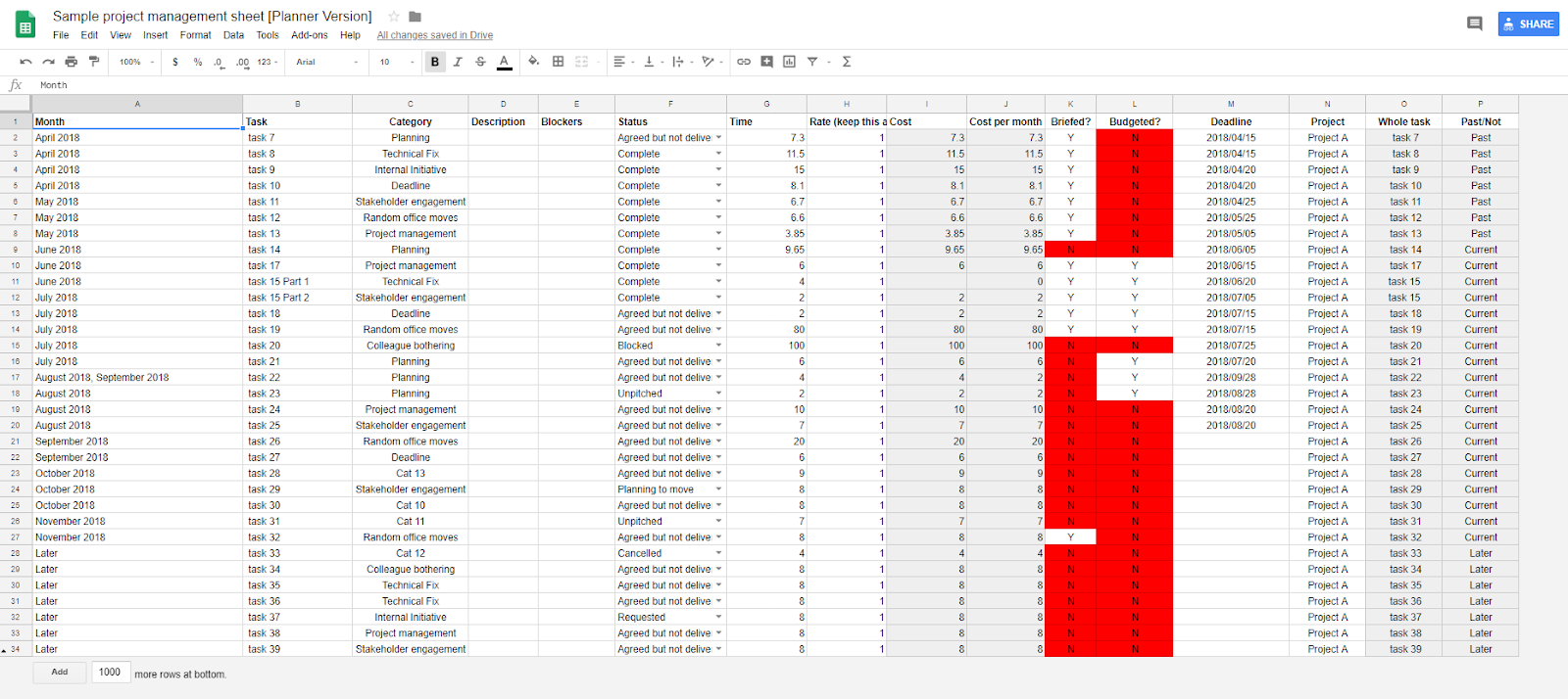
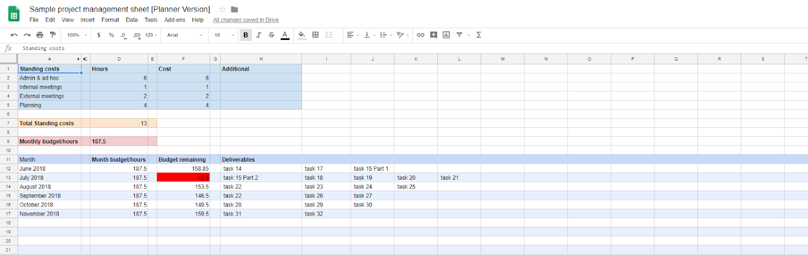
The Planner Version sheet aims to solve this in a few ways. First, you write all the tasks down in the Task View tab, the time period you’re completing them in is on the far left (in my example, it’s the month the task is planned for), and there are other columns like status and category — but initially, it can just be a brain dump of what needs to happen. The idea here is that when you’re first writing everything out, you don’t have to think too much about it — you can easily change the dates and add other information later.
The Month View tab takes the information in the Task List tab and reorders it by the months listed in column A of the Task View (it could be other time periods, as long as it’s consistent).
This way you can look at a time period, see how much resource is left, and read everything you currently have planned (the remaining resource calculation will also take into account recurring tasks you don’t always want to write out, like meetings).
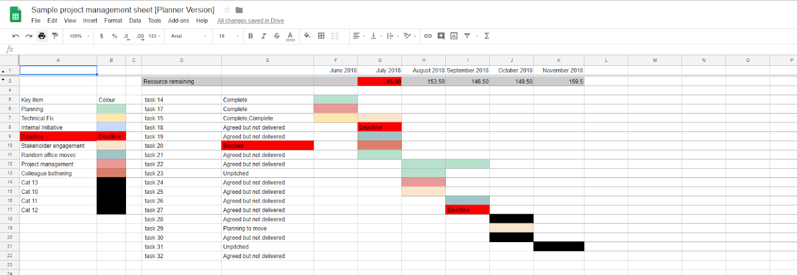
While the Month View tab can help you focus on specific time periods, it doesn’t give you a long-term view of the plan or task dependencies, so we have the two Gantt views. The Gantt View tab contains everything from sixty days ago and into the future, as long as you haven’t just marked the task as “Later.” The Category-Filterable Gantt only focuses on things that are planned for the next six months.
As the name suggests, you can filter this second Gantt to only show specific categories (you label tasks with categories in the Task View tab). This filter is to help with broader trends that are harder to notice — for instance, if the most important part of the project is a social campaign or a site change and you don’t get to it for six months, you may need to make sure everyone is aware of that and agrees. Likewise, if you need to be showing impact but spend most of your time reporting, you may want to change your plan or make sure everyone understands why things are planned that way.
Principle 2: No one knows everything (and they shouldn’t).
If you’re working on a project where you have all the information, then one of two things is likely happening:
- You’ve really doubled down on that neuroticism we share
- You’re carrying this thing — you should just quit and start your own company selling beads* or something.
We can trust that our clients/bosses have more context than we do about wider plans and pressures. They may know more about wider strategies, that their boss tenses up every time a certain project is mentioned, or that a colleague hasn’t yet announced their resignation. While a Google Sheet is never an acceptable substitute for actual communication, our clients or bosses may also have an idea of where they want the project to go which they haven’t communicated, or which we haven’t understood.
We can also trust that people working on individual tasks have a good idea of whether things are going to be a problem — for instance, if we’re allowing far too little time for a task. We can try to be as informed as possible, but they’re still likely to know something we don’t.
Even if we disagree that certain things should be priorities or issues, having a transparent, shared plan helps us kick off difficult conversations with a shared understanding of what the plan currently is. The less everyone has to reprocess information to understand it (see Principle 1), the more likely we are to weed out problems early.
This is all well and good, but expecting someone to absorb everything about a project is likely to have the opposite effect. We need a source of data that everyone can refer to, without crowding their thoughts or our conversations with things that only we as project managers have to worry about.
That’s why we have the Stakeholder Version of our sheets. When we write everything in the Planner Version, the Planned tab is populated with just the things that are relevant for people who aren’t us (i.e, all the tasks where the status isn’t “unpitched,” “cancelled,” “forgotten,” or blank) with none of the resource or project identifier information.
We never have to fill out the Stakeholder Version sheet — it just grabs that information from the Planned tab using importrange() and creates all the same Gantt charts and monthly views — so we don’t have to worry about different plans showing different information.


*Bees?
Principle 3: I’m going to miss stuff (less is more).
I’ll be honest: I’ve spent a bunch of time in the past putting together tracking systems that I don’t check enough. I keep filling them out but I don’t spend enough time figuring out what’s needed where. If we have a Stakeholder Version which takes out the stuff that is irrelevant to other people, we need the same for us. After all, this isn’t the only thing we’re thinking about, either.
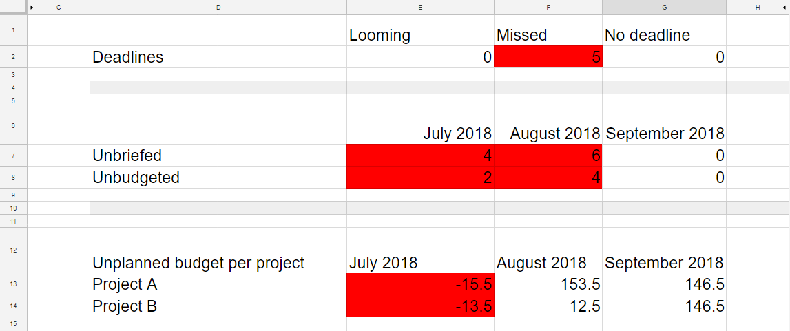
The What-in-God’s-name-have-I-missed Version (God’s-I from now on) pulls in data from all of your individual project management sheets and gives you one place to go to be reminded about all the things you’ve forgotten and messed up. It’s like dinner with your parents in a Google Sheet. You’re welcome.
The three places to check in this version are:
- Alerts Dashboard tab, which shows you the numbers of deadlines upcoming or missed, the work you need to budget for or brief, and how much unplanned budget you have per project, per month (where budget could just be internal people-hours, as that is still finite).
- Task Issues tab, which gives a filterable view of everything over the next three months (so you can dig in to the alerts you see in step one).
- Deadlines This Week tab so you have a quick reminder of what you need to complete soon.
An early conclusion:
Often, when I’m making a point, people tell me they hope I’ll wrap up early. This section is mainly proof of personal growth.
It’s also because everything after this is specific to using, changing, or understanding the project management sheets I’ve shared, so you need only read what follows if you’re interested in how to use the sheets or how I made them (I really do recommend dabbling with some uses of filter() and query(), particularly in conjunction with RegEx formulas).
Aside from that, I hope you find these resources useful. I’ve been getting a lot of value from them as a way to plan with people collaboratively and separate the concept of “project manager” from “person who needs to know all the things,” but I would be really interested in any thoughts you have about how to improve them or anything you think I’ve missed. Feel free to comment below!
Access the template sheets here:
- Planner Version (everything you need to know, plus Gantts)
- Stakeholder Version (a cleaner version for bosses, clients, or people doing the work but not project managing)
- What-in-God’s-name-have-I-missed Version (combined view of lots of different projects, showing you if you’ve forgotten to tell someone about work, missed a deadline, or over-planned)
Appendices & instructions
Some general notes
Quick notes on avoiding problems:
- Make sure that when you copy the sheets, the sharing permissions for the Planner View is email- or at least organization-based (anyone with access to the Stakeholder View will see the Planner View URL). It’s a good idea to keep the God’s-I Version permissions email-based, too.
- Try to follow the existing format of words and numbers as closely as possible when creating new information.
- If you want a new row, I’d insert a row, select the one above, copy it down into the new row, then change the information — that way, the formulas in the hidden columns should still work for you.
- If you want a new column, it might break one of the query() functions; once you’ve added it, have a quick look for formulas using =query() and consider changing the columns they reference that will have been affected by your change.
Quick notes on fixing problems:
Here’s a list of things to check for if you’ve changed something and it isn’t being reflected in the sheet:
- Go through all the tabs in the stakeholder view and unhide any hidden columns
- They usually just contain a formula that reformats text so our lookups work. See if any of those are missing or broken.
- Try copying the formulas from the row above or next to the cell that isn’t working.
- Try removing the =iferror portion of formulas.
- A lot of the cells are set up to be blank if they break. It makes it easier to read the sheet, but can make it harder to know whether something is actually empty or just looks empty.
- If one sheet isn’t properly pulling through data from another, look for the =importrange() formulas and make sure there is one that matches the URL of the sheet you’re trying to reference and that you’ve given permission for the formula to work — you’ll need to click a button.
- Check the Task View tab in the Stakeholder Version and Project URLs tab in the God’s-I Version
- Have you just called a task “Part 4” or similar? There is a RegEx formula which will strip that out.
- Have you forgotten to give a task a type? If so, the Gantt view will warn you in the Status column.
The query function
The =query() function in Google Sheets is awesome — it makes tons of things tons easier, particularly in terms of automating data manipulation. Most of what these sheets do could be achieved with =query, but I’ve often used =filter (which is also very powerful) because =filter is apparently quicker in Google Sheets and at times these sheets have a lot to process.
RegEx
You shouldn’t need to know any RegEx for this sheet, but it is useful in general. Here the RegEx is mainly used to remove the “Part #” in multi-part tasks (see below) and look for anything that matches multiple options — for instance, when selecting multiple categories in the Category-specific forward-facing Gantt tab (see below). RegEx is only used here in RegExmatch(), RegExextract(), RegExreplace(), or as part of the query function where we say “matches.”
Query/filter and isblank
A lot of the formulas in these sheets are either filter() or query() or are wrapped in =if(isblank() — that’s basically because filter and query functions can fill more cells than just the one you put the formula in. For example, they can fill a whole row, column, or sheet. That means that other cells are calculating or looking up against cells which may or may not be empty, so I’ve added the isblank() check so that the cells don’t break when there isn’t information somewhere, but as you add information you don’t have to do as much copying and pasting of formulas.
Tick boxes
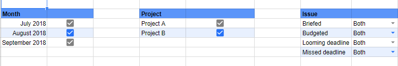
The tick boxes are relatively new in Google Sheets. If you need another one, just copy it from an existing cell or select from the “Insert” menu. Where I’ve used tick boxes, I often have another formula in the sheet which filters rows based on what boxes are ticked, then creates a RegEx based on the values that have a tick next to them.
You don’t need to understand this to use the sheets, but you can see it in the rows I’ve unhidden in the Category-specific forward-facing Gantt tab of the Stakeholder Version sheet.
Quick tip — if you want to change all the boxes to ticked/unticked and don’t want to have to do so one by one, you can copy a ticked or unticked checkbox across all the other cells.
How to add tasks to the list
In the task view, the most important things to include are the task name, time period it’s planned for, cost, and type.

For ease, when creating a new task I recommend inserting a row, copying the row above into it, and then changing the information, that way you know you’re not missing any hidden formulas.
Again, don’t bother changing the Stakeholder Version. Once you’ve added the URL of the Planner Version to the =importrange() function, it will pull automatically from the Planner Version.
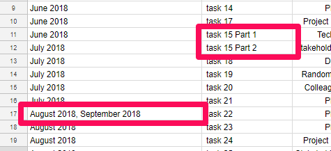
Splitting tasks across multiple time periods
You can put more than one thing in the time period for a task, just by separating it with “, “ (comma space). That’s because when we get the full list of months, we join all the individual cells together with “, “ then split them apart by “, “ and then dedupe the list — so multiple months in one cell are treated the same as all the other months.
=unique(transpose(split(JOIN(", ",'Task view'!A:A),", ",0)))
The cost-per-month formula in the Task List tab counts how many commas are present in the month column for that row, then divides the planned cost by that number — meaning the cost is split equally across all of the months listed.
=H2/(len(REGEXREPLACE(A2,"[^\,]*",""))+1)
If you don’t want the task to be completely equally split between different time periods, you can write “Part 1” or “Part 2” next to a task. As long as you write just “Part” and then numbers at the end of the name, that’ll be stripped out in column O of the task list tab so the different parts of a task will be combined into one record in things like the Gantt chart.
=REGEXREPLACE(B2,"Part \d+$","")
Working with the Month View tab (Planner and Stakeholder version)
A few key things are going on in the Month View tab. First, we’re getting all of the time periods we have listed in the Task View.
Because the months don’t always show up in the right format (meaning later filters don’t work), we then use a =text() formula in the hidden column B to make sure the months stay in the format we need.
Then, in the “deliverables” section of this tab, we use the below formula:
=if(not(isblank(A12)), iferror(TRANSPOSE(FILTER('Task view'!B:B,RegExmatch('Task view'!A:A,B12))),""),"")
What we’re doing above is checking if the “month” cell of this row is has anything in it. If there is a month there, we filter the tasks in the Task View to only those that contain that month in the text month column. Then we use the transpose() function to change our filtered tasks from a vertical list to the horizontal list we see in the sheet.
Finally, we use the below formula to filter the costs we’ve listed in the Task View tab, the same way we filtered the task names above. Then we add together all the costs for the month (plus the standing monthly costs) and subtract them from the total amount of time/hours we have to spend. That way we calculate how much we have left to play with, or if we’re running over.
=if(isblank(A12),"",((D12-SUM(FILTER('Task view'!I:I,RegExmatch('Task view'!A:A,B12))))-sum($D$6:$F$8)))
We also pull this value through to our God’s-I Version to see at a glance if we’ve over/under-planned.
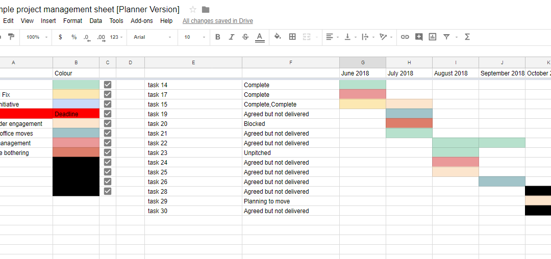
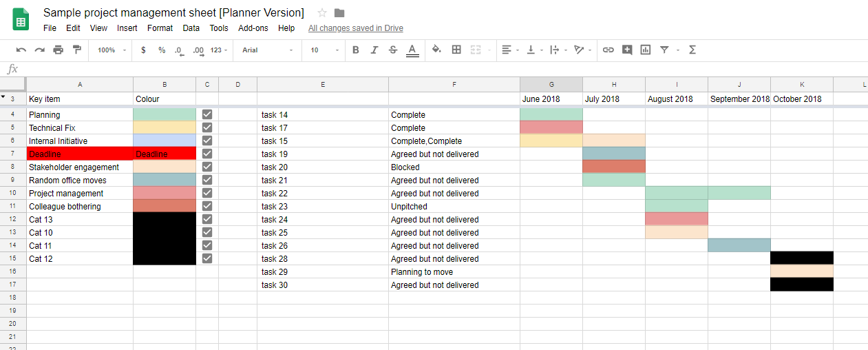
How to make the Gantt charts work (and add categories)
Column C in the Task View tab is the category; you also need to fill this out for the Gantt charts to work. I haven’t forced the kind of categories you have to use because each project is different, but it’s worth using consistent categories (down to the capital letter) because we deduplicate the task categories, and that relies on all of the names being consistent.
What’s happening in the Gantt chart is each cell is a combination of a filter and vlookup (the below looks more complicated than it is).
=iferror(if(not(or(isblank($D6),ISBLANK(F$1))),vlookup(filter('Task view'!$C:$C,'Task view'!$O:$O=$D5,REGEXMATCH('Task view'!$A:$A,F$2)),'Status and colour code'!$C:$E,3,0),""),"")
The formula first checks if the task or month cells are blank. If not, it looks in the month cell in its column and cross-references with the task cell in its row. Where the intersection of a month and task matches a task in our Task View (as in the task in that row is taking place during the month in that column), the filter formula will return the category. For those interested, this might also have been achieved with index-match, but filter lets us match with RegEx so we can give multiple matching options and they don’t have to match exactly. Because we split tasks across multiple months, we need to be flexible in our matching.
The reason we check whether the task or month cells are empty, as mentioned above is so we can paste the above formula in all the cells of the Gantt chart and have them fill out as we add more months and tasks, rather than having to copy and paste the formula each time.
When our filter formula returns the specific category of our task, we take that value and run a vlookup in the Status and color code tab. (That’s only necessary so I could set up the conditional formatting for you so it won’t break when you change the specific category names.)
At the moment, the Gantt charts are set up to color-code the first 7 categories, plus a Deadline category if needed. If you want to add more, they’ll show up initially in the Gantt chart as a black block and you’ll need to set up conditional formatting to color-code them.
To add automatic color formatting for more categories, repeat the below process for each of the Gantt chart views in the Planner and Stakeholder sheets:
- Select all the cells in the tab
- Select “Conditional Formatting” from the Format menu
- Find the rule with the black box next to it and make a note of what number it’s currently targeting from
- Create a new rule for anything which equals the number in step 3, then set the same color for both the background and text of that rule
- Change the rule that’s got a black block next to it to target one number higher
How to make the Category-Filterable Gantt Charts work
This tab uses our old friends, the =filter() and =query() functions. First we use filter to grab the full list of categories from the Status and color code tab we mentioned before:
=FILTER('Gantt view'!A6:B,RegExmatch('Gantt view'!A6:A,".*[a-zA-Z].*"))
Then we put Google Sheets’ shiny new checkboxes next to them (that’ll help us filter our data easily).
Normally we’ll hide row one, but it’s visible to show you a formula that looks at all of the categories and filters them to just those where the tick-box next to them is ticked. If there are none, it returns “(\d|Deadline)” meaning “either a number, or the word Deadline” in RegEx-speak (so anything in our list), because the vertical pipe “|” means “or” and “\d” means “number.”
If there is a tick next to one or more of the categories, the formula will return those things, separated with the “|” that, again, means “or” in RegEx.
=if(countif(C3:C,True)>0,CONCATENATE("(",JOIN("|",FILTER(B3:B,C3:C=True,not(isblank(B3:B)))),")"),"(\d|Deadline)")
Then in cell E3 we have a query formula. The reason we’re using =query and not =filter here is that we need to look for things in more than one column; filter can only really handle one column at a time.
The query function then checks the first six columns of our original Gantt chart, each time looking for any of the category numbers we’ve ticked (what the conditional formatting hides is that the category numbers are in that original Gantt, they’re just the same color as the cell shading). When no tick-boxes are checked, it returns anything that has falls in to any category over the next six planned months. Once we start ticking checkboxes, this will return only the things over the next six planned months that are in one of the categories we’ve selected.
=query('Gantt view'!D1:1056,"Select D, E, F, G, H, I, J where D <> '' and (E matches '"&B1&"' or F matches '"&B1&"' or G matches '"&B1&"' or H matches '"&B1&"' or I matches '"&B1&"' or J matches '"&B1&"')",1)

How to create the Stakeholder View
The Planner Version sheet has a tab called Planned. You don’t need to fill out this tab — it has a query which extracts information from the Task View tab using a =query() function:
=QUERY({'Task view'!A1:F,'Task view'!O1:P},"Select * where not (Col6 contains 'pitched' or Col6 contains 'cancelled' or Col6 = '' or Col6 = 'Forgotten')")
All the formula above is doing is taking the Month, Task, Description, Blocker, Status, Category, and Full task columns, then showing every record where the status isn’t “unpitched,” “cancelled,” “forgotten,” or empty. That gives us a tab with the information we’re ready to share. We could also achieve this with =filter() if we reordered the data in the Task View tab, but this ordering of data is easier to work with, so we just use =query() and select only the columns we want here, combining the ranges horizontally by listing them between {} at the start of this formula.
Then, the Task View tab in our Stakeholder Version sheet file uses =importrange() to target that cleaned list we’ve created. To make sure the Stakeholder Version keeps functioning when you create copies of both of these files, all you need to do is go to the new Planner Version sheet and copy the URL of the page, then go to the Stakeholder Version, find the Task View tab, and update the importrange() formula in cell A1 to have the new URL of your Planner Version sheet. The cell will recalculate, you’ll need to grant permission, then it should work as normal.
How to update the God’s-I Version
This view gives you the following:
A quick look at the total number of tasks in any project which:
- Have a deadline within 10 days of now
- Have passed a deadline (with the task not completed)
- Don’t have a deadline set
- Aren’t briefed or aren’t budgeted for the next three months
It’ll also give you a quick look at the amount of unplanned budget per project, per month, to make sure you haven’t forgotten to plan a month and haven’t overplanned a month.
The God’s-I Version works in a similar way to the Stakeholder Version in that it pulls in information using =importrange(), but a key difference is that we want to pull from multiple sheets. Rewriting the formula could get to be a pain, so instead we can generate the formula we need in the Project URLs tab.
The only things you need to do are:
- Add the URL of the new Planner View sheet you want to include in the Project URLs tab of the God’s-I Version
- Grant permission for this sheet to access that sheet (you can click on the alert that appears in column A)
- Copy the value in Cell B1, go to the All Imported Task Views tab and select cell A2, then paste the value into the top bar. It’s important that we don’t paste straight into the cell or the sheet will run the concatenate formula rather than the query formula we’re making.
It’s worth noting that this sheet will have all the information about every project you’re managing. Once it’s set up, you shouldn’t share access to anyone unless you’re happy with them seeing all the budgeting details for each of the sheets.
A late conclusion:
Why are you looking for a conclusion down here? It’s in the middle of the post under the title of “An early conclusion,” of course. Have a nice day!
Sign up for The Moz Top 10, a semimonthly mailer updating you on the top ten hottest pieces of SEO news, tips, and rad links uncovered by the Moz team. Think of it as your exclusive digest of stuff you don’t have time to hunt down but want to read!
![]()